sympy is a great tool for symbolic computations developed in Python. It has a module for differential geometry that allows you to compute some of the important objects as the Christoffel symbols and curvature objects. I wanted to give it a try and I created a jupyter notebook with a simple test using the Schwarzschild metric and numerically computing some geodesics.

1
2
3
4
5
6
7
8
9
10
11
12
13
14
15
16
17
18
19
20
21
22
23
24
25
26

%matplotlib inline

# General imports
from itertools import product
import matplotlib
import numba
import numpy as np
import matplotlib.pyplot as plt
from IPython.display import display, Math

# Basic imports and functions
from sympy import latex, symbols, sin, cos, pi, simplify, lambdify, Matrix
from scipy.integrate import solve_ivp



from sympy.diffgeom import (
    Manifold,
    Patch,
    CoordSystem,
    metric_to_Christoffel_2nd,
    TensorProduct as TP
)

def lprint(v):
    display(Math(latex(v)))

Create now the coordinate system to define the metric as:

\[ c^2 \diff{\tau^2} = \left(1 - \frac{r_s}{r}\right) c^2 \diff{t^2} - \left(1 - \frac{r_s}{r}\right)^{-1} \diff{r^2} - r^2 \left(\diff{\theta^2} + \sin^2(\theta) \diff{\phi^2} \right) \]

1
2
3
4
5
6
7
8
9
10
11
12
13
14
15
16
17
18
19
20
21
22
23
24
25
26
27
28
29

# Create a manifold.
M = Manifold('M', 4)

# Create a patch.
patch = Patch('P', M)

# Basic symbols
c, r_s = symbols('c r_s')

# Coordinate system
schwarzschild_coord = CoordSystem('schwarzschild', patch, ['t', 'r', 'theta', 'phi'])

# Get the coordinate functions
t, r, theta, phi = schwarzschild_coord.coord_functions()

# Get the base one forms.
dt, dr, dtheta, dphi = schwarzschild_coord.base_oneforms()

# Auxiliar terms for the metric.
dt_2 = TP(dt, dt)
dr_2 = TP(dr, dr)
dtheta_2 = TP(dtheta, dtheta)
dphi_2 = TP(dphi, dphi)
factor = (1 - r_s / r)

# Build the metric
metric = factor * c ** 2 * dt_2 - 1 / factor * dr_2 - r ** 2 * (dtheta_2 + sin(theta)**2 * dphi_2)
metric = factor * c ** 2 * dt_2 - 1 / factor * dr_2 - r ** 2 * (dtheta_2 + sin(theta)**2 * dphi_2)
metric = metric / c ** 2

1
2

# Get the Christoffel symbols of the second kind.
christoffel = metric_to_Christoffel_2nd(metric)

1
2
3
4

# Let's print this in an elegant way ;)
for i, j, k in product(range(4), range(4), range(4)):
    if christoffel[i, j, k] != 0:
        display(Math(f'\Gamma^{i}_{{{j},{k}}} = ' + latex(christoffel[i, j, k])))

\[ \Gamma^0_{0,1} = \frac{r_{s}}{2 \mathbf{r}^{2} \left(1 - \frac{r_{s}}{\mathbf{r}}\right)} \]

\[ \Gamma^0_{1,0} = \frac{r_{s}}{2 \mathbf{r}^{2} \left(1 - \frac{r_{s}}{\mathbf{r}}\right)} \]

\[ \Gamma^1_{0,0} = - \frac{r_{s} \left(- c^{2} + \frac{c^{2} r_{s}}{\mathbf{r}}\right)}{2 \mathbf{r}^{2}} \]

\[ \Gamma^1_{1,1} = \frac{c^{2} r_{s} \left(- c^{2} + \frac{c^{2} r_{s}}{\mathbf{r}}\right)}{2 \mathbf{r}^{2} \left(c^{2} - \frac{c^{2} r_{s}}{\mathbf{r}}\right)^{2}} \]

\[ \Gamma^1_{2,2} = \frac{\mathbf{r} \left(- c^{2} + \frac{c^{2} r_{s}}{\mathbf{r}}\right)}{c^{2}} \]

\[ \Gamma^1_{3,3} = \frac{\mathbf{r} \left(- c^{2} + \frac{c^{2} r_{s}}{\mathbf{r}}\right) \sin^{2}{\left(\mathbf{\theta} \right)}}{c^{2}} \]

\[ \Gamma^2_{1,2} = \frac{1}{\mathbf{r}} \]

\[ \Gamma^2_{2,1} = \frac{1}{\mathbf{r}} \]

\[ \Gamma^2_{3,3} = - \sin{\left(\mathbf{\theta} \right)} \cos{\left(\mathbf{\theta} \right)} \]

\[ \Gamma^3_{1,3} = \frac{1}{\mathbf{r}} \]

\[ \Gamma^3_{2,3} = \frac{\cos{\left(\mathbf{\theta} \right)}}{\sin{\left(\mathbf{\theta} \right)}} \]

\[ \Gamma^3_{3,1} = \frac{1}{\mathbf{r}} \]

\[ \Gamma^3_{3,2} = \frac{\cos{\left(\mathbf{\theta} \right)}}{\sin{\left(\mathbf{\theta} \right)}} \]

Solving the geodesic equation.

The geodesic equation is

\[ {d^{2}x^{\mu } \over ds^{2}}+\Gamma ^{\mu }{}_{\alpha \beta }{dx^{\alpha } \over ds}{dx^{\beta } \over ds}=0 \]

The term \( x^\mu \) is a path depending on \( s \).
Let \( u(s) = x(s) \) and \( v(s) = \dot{u}(s) \), then we can translate the geodesic equation into the equations

\[ \dot{u}^\mu(s) = F^\mu_1(u(s),v(s)) \]

and

\[ \dot{v}^\mu(s) = F^\mu_2(u(v), v(s)) \]

with

\[ F^\mu_1(u(s),v(s)) = v^\mu(s) \]

and

\[ F^\mu_2(u(s), v(s)) = - \Gamma^\mu_{\alpha \beta} v^\alpha(s) v^\beta(s),. \]

1
2
3
4
5
6
7
8
9
10
11
12
13
14

g_func = lambdify((c, r_s, r, theta), christoffel, modules='numpy')

## Specify c and r_s
def F(t, y):
    u = np.array(y[0:4])
    v = np.array(y[4:8])

    chris = g_func(1, 1, u[1], u[2])

    du = v
    dv = -np.dot(np.dot(chris, v), v)

    return np.concatenate((du, dv))

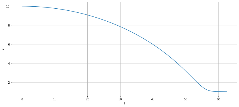
Use the method solve_ivp of sympy to compute numerically the geodesic starting at the event \( (t,r,\theta, \phi) = (0, 10, \frac{\pi}{2}, 0) \) in the direction of the tangent vector \( (1, 0, 0, 0) \).

1
2
3
4
5
6
7
8
9
10
11
12
13
14
15

T = 70
t_eval = np.linspace(0, T, int(T * 123 + 1))
initial_value = [0, 10, np.pi/2, 0, 1, 0, 0, 0]

# Solve the initial value problem.
sol = solve_ivp(F, [0, T], initial_value, t_eval=t_eval)

# Plot the solution.
plt.figure(figsize=(14, 6),)
plt.plot(sol.y[0], sol.y[1])
ax = plt.gca()
gax.axhline(1, color="red", ls='--', lw=1)
plt.grid()
plt.xlabel('t')
plt.ylabel('r')